- Analytical methods
-
PLA 3.0
- About PLA 3.0
-
Analyze your data
- Analyze Biological Potency Assays
- Analyze quantal response assays
- Analyze the dose-response relationship
- Analyze the endotoxin concentration in a substance
- Develop Equivalence margins
- Determine the potency of antibiotics
- Perform a curve comparisons
- Perform a Linearity-of-dilution assessment
- Perform a sophisticated statistical process control
- Perform combination calculations
- Import your data
- Supporting add-ons
- Compliance features
- Deployment
- Try & Buy
- PLA 3.0 Academy
- Support
- Company
Analyze the dose-response relationship
The Dose-Response Analysis Package (available as a free add-on) provides a range of additional biostatistical methods (Content Assays) for immunoassays, ELISA, and more. It supports you in investigating equivalence for calibration curves and it provides enhanced data processing and analysis. New document reports and dashboards add to its value and usability.
Biostatistical methods in the Dose-Response Analysis Package
The biostatistical methods of the package include :
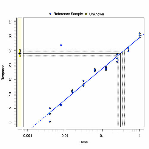
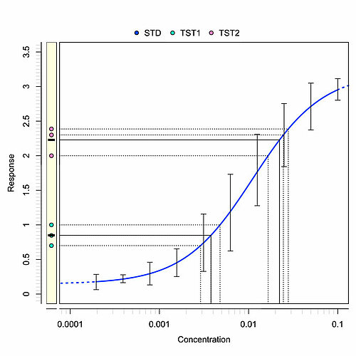
- Interpolation on calibration curves
- Spike-and-recovery analysis
- Linearity-of-dilution assessment
- Effective-concentration calculation (EC50)
- Curve comparisons
- Equivalence margin development
- The package features several equivalence test and development options for calibration curves. You can employ equivalence and point estimate tests for parameter estimates and ANOVA terms. And you can use your historic assay runs to develop acceptance criteria. The package provides test strategy development, visualizations, and simulations.
Response data processing and subgroup analysis
The package also features enhanced response data processing. You can adjust and normalize data either by a fixed value or by another assay element. Use these features, for example, to subtract the absorbance of blank wells or to divide response values by the mean absorbance of maximum binding wells. You can also employ transformations–logarithmic, square, and square-root. Apply adjustments, normalizations, and transformations to all samples, a specific sample, or to all test or control samples. You can apply adjustments and normalizations to specific plates as well. Moreover, you can average your replicates. To give you full control over data processing, you can employ several adjustment and normalization steps and you can adjust the sequence of response data processing steps to your needs.
With the package, you can define analysis subgroups suitable to your experiment. Subgroups are available for both, single- and multi-dose samples. Use this feature, for example, to group samples in spike-and-recovery analysis or assay optimization. Statistics for interpolated results and dose-response curve characterization include averages, standard deviations, coefficient of variations, and recovery rates. Visualize results in overlay plots.
Document reports and dashboards
New document reports and dashboards further add to the package's value and usability. The dashboards display key attributes of document definitions and calculation results and visualize results in new data plots. The revised design of both reports and dashboards provides greater lucidity with a fresh and modern look, clear, uniformly applied layout, and a uniform color scheme in line with editor. Read more
Please note: The Dose-Response Analysis Package is not intended for relative potency calculations, as those are covered by the Biological Assay Package.
Example Reports
-
Example report of a Effective Concentration Calculation with PLA 3.0 174 KB
This report is intended to show the capabilities of the Dose-Response Analysis Package for PLA 3.0 for calculating effective concentrations. It contains (artificial) observations for one standard sample and two test samples with measurements taken in triplicate at eight concentrations along a two-fold geometric sequence each. For each sample, a four-parameter logistic curve is fitted to the data. Effective concentrations and EC50 ratios are calculated, and suitability tests are evaluated. The three samples in this document also showcase three different ways to define the concentration of a sample: 1. By defining the stock solution of the analyte (Curve 1) 2. By defining the initial concentration of your dilution sequence (Curve 2) 3. By defining the concentration of the raw material used for stock solution preparation (Curve 3)
-
Example report of a Curve Comparison with PLA 3.0 202 KB
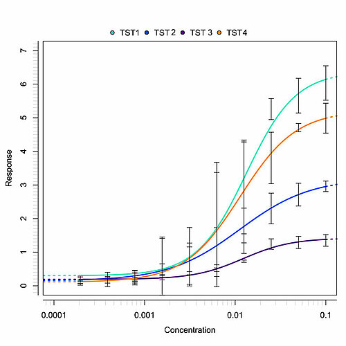
This report is intended to show the curve-comparison capabilities of the Dose-Response Analysis Package for PLA 3.0. It contains (artificial) observations for three samples with measurements taken in triplicate at eight concentrations along a two-fold geometric sequence. For each sample, a four-parameter logistic curve is fitted to the data, and suitability tests are evaluated. All samples are collected in a report group. For this group, an overlay plot is created, and the parameters of the fits are compared. The three samples in this document also showcase three different ways to define the concentration of a sample: 1. By defining the stock solution of the analyte (Curve 1) 2. By defining the initial concentration of your dilution sequence (Curve 2) 3. By defining the concentration of the raw material used for stock solution preparation (Curve 3)
-
Example report of an Interpolation Analysis with PLA 3.0 2 MB
This report shows the interpolation capabilities of the Dose-Response Analysis Package for PLA 3.0. It contains (artificial) observations for a four-parameter logistic standard curve and 75 test samples. The standard is measured at seven concentration steps, with three replicates for each concentration. Each test sample is measured with one replicate. Test samples are interpolated against the standard curve, concentrations are determined, and sample suitability tests are evaluated.
-
Example report of a Linearity-of-dilution assessment with PLA 3.0 426 KB
This report shows how to use the Dose-Response Analysis Package for PLA 3.0 to perform linearity of dilution assessment. It contains (artificial) observations for a standard sample and 12 test samples. The standard is measured along a two-fold geometric sequence with seven steps where each measurement is taken in duplicate. Each test sample is measured in triplicate. The test samples are grouped into three groups of four samples each, corresponding to a serial dilution of three underlying samples representing three different initial concentrations. The concentration of the undiluted (neat) sample is assigned to all diluted samples of its group, and recoveries are calculated and tested. Additionally, all test samples belonging to the same 'neat' sample are collected in a report group, and a combined recovery for each group is calculated.
-
Example report of a Spike-and-recovery analysis with PLA 3.0 839 KB
This report shows how to use the Dose-Response Analysis Package for PLA 3.0 to perform spike and recovery analysis. It contains (artificial) observations for a standard sample, 21 test samples, and seven control samples. The standard is measured along a two-fold geometric sequence with seven steps where each measurement is taken in duplicate. Each test and control sample is measured in triplicates. For each sample matrix, three test samples represent the spiked samples, and one control sample represents the unspiked matrix. Spiked samples are assigned a concentration according to the spike, and recoveries are calculated and tested. Additionally, all test samples with the same spike concentration are collected in a report group, and a combined recovery for each group is calculated.


